Factor Models and Synthetic Control

When I first saw the synthetic control method, I had a really hard time understanding when it would work and when it would not. Sure, you need a lot of pre-periods. But what else? “Good pre-treatment fit”. If I’m thinking about a research question, how can I decide if I’ll have good pre-treatment fit a-priori? Certainly, looking at the results to decide isn’t a good idea (paging Jon Roth).

I sort of stumbled onto factor models in a completely different context. But, after I learnt this model, I began seeing it pop up again and again in papers about synthetic control. They made such a large difference in my understanding that I wanted to share what I’ve learned.

First, I’ll share what a factor model is and then I’ll circle back to how it connects to synthetic controls. As an important disclaimer: the synthetic control estimator is consistent under a wide variety of data-generating processes. However, the factor model is a leading case and it is pedagogically useful.

Factor Models

The simplest factor model is given by

where $\bm f_t$ is a $p \times 1$ vector of unobservable “factors” and $\bm \gamma_i$ is a $p \times 1$ vector of unobservable “factor loadings”. Notice that this kind of looks like a time fixed-effect and a unit fixed-effect, but they’re multiplied together.

We can view the factors $\bm f_t$ as macroeconomic shocks with factor loadings $\bm \gamma_i$ denoting a unit’s exposure to the shocks. The product of the two depics how a unit is affected by the macroeconomic shock. For example, imagine $y$ is GDP. A factor-loading could be a counties’ share of manufacturing employment. The factor could be a common national shock to manufacturing employment (e.g. import competition or other changes to the national economy). The product of the two would be the effect of the national shocks on a given counties’ GDP.

Another possibility lets the $\bm \gamma_i$ represent time-invariant characteristics with a marginal effect on the outcome $\bm f_t$ that changes over time. For example, imagine $y$ is wages. For example, imagine $y$ is a worker’s wage in a given year. A factor-loading could be a worker’s education, $\bm{\gamma}_i$. The factor, $\bm{f}_t$, could be a common national shock to the returns to education (e.g. changes in the national college premium). The product of the two would be the effect of the national shocks on a given worker’s wage.

However, these are just examples of what could be in there. The power of a factor model is that we don’t need to be able to actually measure $\bm{\gamma}_i$ or $\bm{f}_t$ to control for them. Just like with unit and time fixed-effects, you might have ideas on what goes in them, but you don’t actually need to measure them.

Note that the two-way fixed effect is actually an example of a factor model! Take $\bm{\gamma}_i = (1, \mu_i)$ and $\bm{f}_t = (\lambda_t, 1)$; then the model becomes $y_{it} = \lambda_t + \mu_i + u_{it}$. However, the factor model allows for units to be on differential trends (based on their exposure to national shocks).

Since the factor model nests the standard TWFE model, why not just use them in difference-in-differences models?? Well, of course, there’s no free lunch and this model is no exception. The problem is that we need long panels in order to consistently estimate the factors and the factor-loadings seperately (you can’t within-transform them away like you can’t with TWFE model). It turns out, that one powerful way to think about synthetic control is through factor models.

Synthetic Control

The basic idea of synthetic control is to identify a set of control units that “well-approximate” the outcome for the treated unit in the pre-treatment periods. The synthetic control estimator is then the weighted average of the control units. The original synthetic control paper shows that when the outcome model is a factor-model, the synthetic control estimator’s bias goes to 0 when the number of pre-periods are large (to be clear, the synthetic control estimator is consistent under other data-generating processes).

Under a factor model, the synthetic control estimate for the treated unit’s untreated potential outcome is formed as the weighted average of the control unit’s outcomes $\hat{y}_{it}^{sc} = \sum_j w_j y_{jt}$, where $w_j$ are found via the synthetic control procedure. We label the treated unit as $i = 0$. Ignoring the error term, we can write this as

The last term shows the insight, the synthetic control unit’s outcome is generated affected by the same factors and with factor-loadings given as the weighted average of the control units’ factor-loadings.

When does the synthetic control do a good job? Well, when the synthetic control units’ factor-loadings look similar to the treated units factor-loadings, $\bm{\gamma}^{sc} = \bm{\gamma}_0$! If we satisfy this condition, then our predicted counterfactual outcome in the post-periods is good. Intuitively, the synthetic control and the treated unit are subject to the same factor shocks and they have the same “exposure” to those shocks.

I find this interpretation really useful. As a researcher, I can start thinking of these conditions a-priori. First, I think of factors that are important in my setting (e.g. in the GDP example, I think an important confounding shock may be shocks to industries over time.). Second, I think of whether my treated units’ factor-loadings (e.g. their industrial mix) can be well approximated by the donor pool. This would fail in our ongoing example if my treated county is an outlier in terms of their industrial mix.

I’m not sure I’ve seen this recommended anywhere, but it strikes me as a good check to compute weighted averages of important characteristics that you think might be confounders with treatment selection (proxied by baseline covariates $X$) and see if the synthetic control weights approximate the treated units weights, $\sum w_j X_j \approx X_0$.

The last connection I’ll make is about the importance of long panels for estimating synthetic control. In the above work, notice I ignored the error term. That is because, in long panels, the error term becomes zero. But this isn’t true in short panels because the synthetic control procedure ends up matching on noise instead of matching on factor-loadings. That makes the $\bm{\gamma}^{sc} \neq \bm{\gamma}_0$.

Examples of factor-models in synthetic control papers

To see how prevelant the use of factor models are, I’ll end with some examples of their appearance throughout the econometric literature.

1. Ferman and Pinto - Synthetic Control with Imperfect Pre-Treatment Fit

The authors consider what happens when the pre-treatment fit is imperfect deriving results and a new estimator under a factor model.

”We consider the properties of the SC and related estimators, in a linear factor model setting, when the pre-treatment fit is imperfect. We show that, in this framework, the SC estimator is generally biased if treatment assignment is correlated with the unobserved heterogeneity, and that such bias does not converge to zero even when the number of pre-treatment periods is large.”

2. Gobillon and Magnac - Regional Policy Evaluation: Interactive Fixed Effects and Synthetic Controls and Xu - Generalized Synthetic Control Method

Propose an imputation treatment effect estimator that directly estimates the factor-loadings and the factors themselves. This is very similar to the imputation estimator from Borusyak et. al. (2021) and Gardner (2021).

3. Ben-Michael, Feller, and Rothstein - The Augmented Synthetic Control Method

Considers how to use regularization on the weights to prevent over-fitting in shorter panels. This helps better approximate the true treated unit’s factor-loadings in a factor-model.

4. Athey, Bayati, Doudchenko, Imbens and Khosravi - Matrix completion methods for causal panel data models

They impute untreated potential outcomes by estimating a low-rank factor model using nuclear-norm regularization to prevent over-fitting.

Short panels

All of these papers mentioned all rely on long-panels to properly identify the underlying factor structure. Over the last two years, I’ve been working on a research agenda that proposes estimators that remain valid in short-panels.

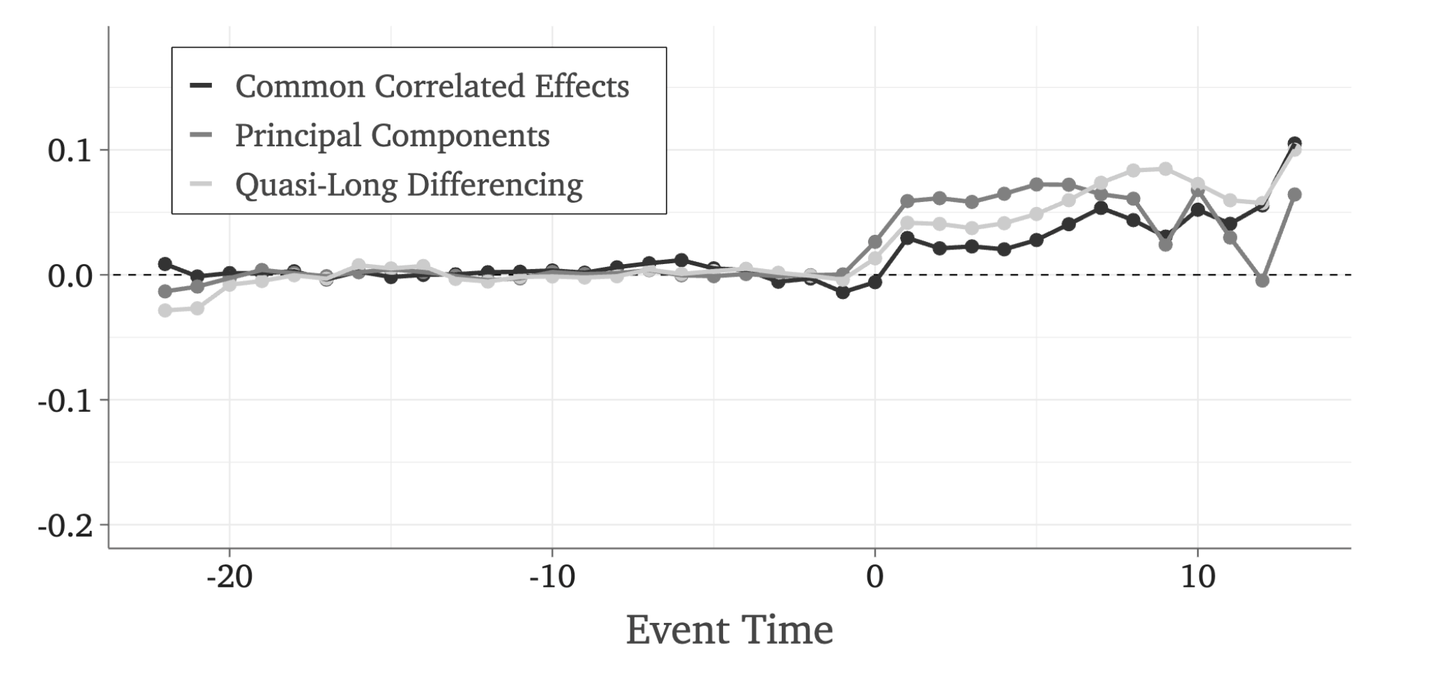
The key insight my coauthors and I have found is that treatment effect estimators only require consistent estimation of $\bm{f}_t$ and not estimation of $\bm{\gamma}_i$ so long as you have many treated units. Using this insight, we have “unlocked” a large econometric literature that shows when $\bm{f}_t$ can be estimated consistenly in short-panels and derived a way to “plug” these estimators into an imputation estimator.

For example, consistently estimates of $\bm{f}_t$ can be estimated by instrumental variables (quasi-long differencing) or by using covariates that are affected by the same factor structure (common correlated effects). Both of these can then be plugged into an estimator that pops out a nice event-study graph. Here’s an example from our paper: