<code>{did2s}</code>: Two-Stage Difference-in-Differences

`{did2s}`: Two-Stage Difference-in-Differences

Kyle Butts and John Gardner

R Journal, 2022

Published|Slides|R Package|Stata Package

We present statistical software to implement imputation estimator for difference-in-differences.

Abstract

Recent work has highlighted the difficulties of estimating difference-in-differences models when treatment timing occurs at different times for different units. This article introduces the R package {did2s} which implements the estimator introduced in Gardner (2021). The article provides an approachable review of the underlying econometric theory and introduces the syntax for the function did2s. Further, the package introduces a function, event_study, that provides a common syntax for all the modern event-study estimators and plot_event_study to plot the results of each estimator.

5-Minute Summary

The standard difference-in-differences estimator is modeled using the Two-way Fixed Effects Model. Unit $i$ and time $t$ has potential outcome:

y_{it} = \mu_i + \eta_t + \tau D_{it} + \varepsilon_{it},

where $D_{it}$ is an indicator variable that equals one when unit $i$ is currently experiencing treatment at time $t$ . Researchers aim to estimate the effects of treatment and summarize it as the Average Treatment Effect on the Treatment, $\tau$ .

If the two-way fixed effects model is correctly specified and the parallel trends assumption is satisfied, then OLS is fine and even BLUE! (woohoo 🎉🎉) So what’s with all these new Diff-in-Diff doesn’t work well problems?

Problem 1: $\tau$ is not constant

The first problem is that $\tau$ is not typically constant across units and over time:

Treatment effects may depend on when you start treatment. For example, groups that benefit more from a policy implement it earlier
Treatment effects may depend on treatment duration like an event-study. For example, policy effects slowly take hold as the policy is adopted broadly.

Our TWFE model clearly needs to be enriched:

y_{it} = \mu_i + \eta_t + \tau_{gt} D_{it} + \varepsilon_{it},

where now we have what the literature calls the Group-Time Average Treatment Effect, $\tau_{gt}$ . This captures the two forms of treatment effect heterogeneity described above. The treatment effect size to depend on when you are treated, group $g$ , and how many periods it has been since treatment determined by $t - g$ . It will prove really hard to accurately estimate any particular $\tau_{gt}$ , so researchers will try to estimate the Overall Average Treatment Effect:

\tau \equiv \frac{1}{N_{gt}}\sum \tau_{gt},

the average of $\tau_{gt}$ across all $(g,t)$ observed in the sample.

Estimating Overall Average Treatment Effect

If we knew $\mu_i$ and $\eta_t$ , then we could move terms around in our model and have:

y_{it} - \mu_i - \eta_t = \tau_{gt} D_{it} + \varepsilon_{it}.

Then, if we ran this regression of an outcome variable ( $y_{it} - \mu_i - \eta_t$ ) on an indicator variable $D_{it}$ , then OLS algebra says that $\hat{\tau}$ will take the average of $\tau_{gt}$ for us and estimate the overall average treatment effect $\tau$ .

Too bad we don’t know $\mu_i$ and $\eta_t$ … Since we don’t know them, why don’t we instead estimate them? From the Frisch-Waugh-Lovell (FWL) theorem, we have:

y_{it} - \hat{\mu}_i - \hat{\eta}_t = \tau_{gt} \tilde{D}_{it} + \varepsilon_{it},

where everything looks about the same, but now $\hat{\mu}_i$ and $\hat{\eta}_t$ are estimated and $\tilde{D}_{it}$ is the treatment indicator after being residualized by unit and time fixed effects. The left-hand side is a good estimate for $\tau_{gt}$ , so what’s the problem then? This residualized treatment variable is actually the source of all the problems you’ve heard about. No really, go look at the proofs in those papers, you’ll see $\tilde{D}_{it}$ right away.

The problem is that since $\tilde{D}_{it}$ is no longer a simple dummy variable, OLS no longer estimates the simple average of $\tau_{gt}$ .

Instead, OLS estimates

\hat{\tau} = \sum w_{gt} \tau_{gt} \neq \tau,

where the weights $w_{gt}$ are quite strange, but sum to 1. I’ll leave it to the paper to describe the weights, but no this: In some cases, $\hat{\tau}$ can be the opposite sign of the overall average treatment effect, $\tau$ 🚩🚩!

Okay, so why don’t you just regress $y_{it} - \hat{\mu}_i - \hat{\eta}_t$ on $D_{it}$ ? Great idea! You just thought of the two-stage difference-in-differences estimator (and Borusyak et. al.’s estimator too)

Two-stage Difference-in-Differences estimator

The above intution (hopefully) has lead us directly to the two-stage differences estimator as proposed by Gardner (2021). The two stages are as follows:

Stage 1: Estimate $\mu_i$ and $\eta_t$ using untreated/not-yet-treated observations ( $D_{it} = 0$ ). Don’t include $D_{it} = 1$ since the treatment effects will be partially absorbed by unit and time fixed effects.
Stage 2: Regress $y_{it} - \hat{\mu}_i - \hat{\eta}_t$ on $D_{it}$ , not $\tilde{D_{it}}$ !.

Inference is a bit more complicated in this two-step estimator since your “outcome variable” is a noisy estimated object. Valid inference needs to account for this first-stage estimation. The details are in the paper and done properly in the {did2s} package.

`{did2s}`

The paper then goes on to show off the {did2s} package and provide some practical advice when implementing the estimator. For example, we will show how {did2s} works for a dataset of simulated data with a treatment effect of 2.

library(did2s)
data("df_hom")

static = did2s(
  df_hom,
  yname = "dep_var", treatment = "treat", cluster_var = "state",
  first_stage = ~ 0 | unit + year,
  second_stage = ~ i(treat, ref=FALSE),
  verbose = TRUE
)

Running Two-stage Difference-in-Differences
• first stage formula `~ 0 | unit + year`
• second stage formula `~ i(treat, ref = FALSE)`
• The indicator variable that denotes when treatment is on is `treat`
• Standard errors will be clustered by `state`

Since the package returns a fixest object, you can use the suite of exporting tools that fixest provides, like esttable and iplot/coefplot. This makes, for example, exporting latex tables and event-study plots super simple.

fixest::etable(static)

                           static
Dependent Var.:           dep_var

treat = TRUE    2.025*** (0.0307)
_______________ _________________
S.E. type                  Custom
Observations               31,000
R2                        0.31846
Adj. R2                   0.31846

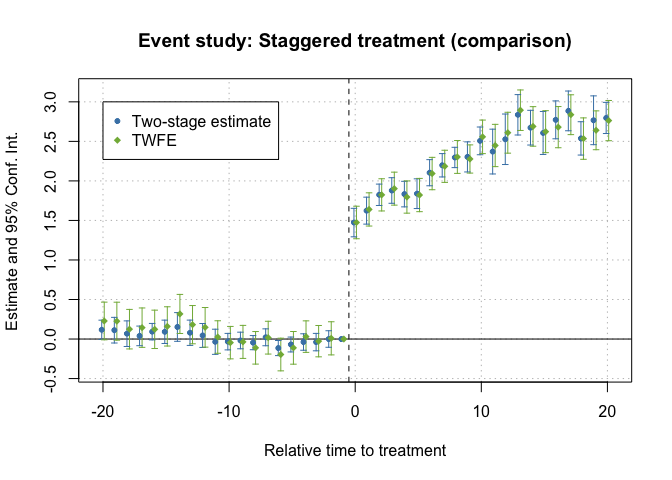
Alternatively, if we use relative year indicator variables in the second-stage, we estimate event-study type coefficients.

dynamic = did2s(df_hom,
    yname = "dep_var", treatment = "treat", cluster_var = "state",
    first_stage = ~ 0 | unit + year,
    second_stage = ~ i(rel_year, ref=c(-1, Inf)),
    verbose = FALSE
  )

Then, plutting an event study is super simple with fixest::coefplot.

# plot rel_year coefficients and standard errors
fixest::coefplot(dynamic)

**Figure:** Two-stage Difference-in-Differences

{did2s}: Two-Stage Difference-in-Differences